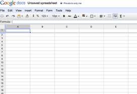
A spreadsheet stores, organizes, and performs calculations on data. Creating a spreadsheet is the same as adding a text document. Find the Create button in the upper left corner of the interface and select Spreadsheet from the drop-down list. Then a blank sheet opens in a new browser tab.
Google Spreadsheets includes many of the same options as Google Docs. To change the title, click on the Untitled spreadsheet box at the top. All the changes are automatically saved in a short periods of time.
Toolbar
Spreadsheets editor also features a toolbar above the placeholder. It is a bit more complicated than in text documents, but still user-friendly and transparent. The first array of icons includes Print, Undo, Redo, and HTML formatting.
At this point, it is worth mentioning what is the last command for. Well, it allows you to copy not only the text itself, but its appearance including font, color, bold or underlines. These parameters can then be applied to a new text or spreadsheet cell.
The second array of icons from the left makes it easy to define the content of the cell. We can specify whether the inserted number is the amount (Format as currency) or percent (Format as a percentage). The button with numbers 123 provides additional formatting options.
How does it work? If you enter into a cell number 112, and then you select the command Format as currency, the service will automatically change the entry to 112.00. We do not need not determine the number of decimal points.
Merging and text flow
Other icons represent the very basic options, these include: the font ( 6 fonts to choose from), size, bold (Ctrl + B), italic (Ctrl + I), underline, text color and fill color (changes the color of the selected cells). Another icon lets you add borders to the selected cells.
One of the most useful options is the ability to merge several cells into one cell. Previously, there was a function for merging cells horizontally, but it worked pretty badly. Now we can use the same icon to connect the elements horizontally or vertically.
The next block of icons is related to the text flow. We have a plenty of choice, such as align to the left, align to the middle, align to the right, align at the top, align at the bottom, as well as change the vertical and horizontal alignment of the selected cell’s contents. The third icon lets you wrap text – and it is enabled by default.
Due to this, the cell’s contents will not protrude from the right side of the neighboring fields. Instead, you get a few lines of text, which can be fully visible if you increase the height of the field. Last but not least icon allows you to insert comments (I wrote about this in the article about word processing), graphs and functions.
Menu with commands
In addition to the toolbar, users are provided with a menu similar to the one in LibreOffice Calc or MS Excel. Most of the components cover the range of options from the editor. Noteworthy is the Data menu, which allows you to sort the contents of the entire worksheet, select them in alphabetical order or the other way round.
The Tools menu comes bundled with more options, featuring the Gallery Script - plugins that increase the functionality of the spreadsheet editor. There's also the possibility to protect a document, or disable AutoComplete option. The Help menu includes a complete list of keyboard shortcuts.
How to create charts?
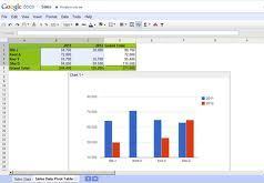
When it comes to designing charts, it is another feature that has a strong resemblance to those found in Microsoft Excel. To start with, enter your data into rows, then select the cells and click on the Chart button in the toolbar.
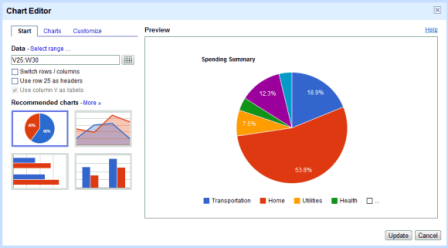
From this point, we can modify the range of the table, select the type of chart, such as bar or pie, add a title and the horizontal and vertical axis, and adjust the font color and graphics, change or reverse the position of the legend. Once you are satisfied with your work, click on Save chart. If you want to edit the chart, choose Edit chart from the
Menu, and select the element you want to edit.
How to use formulas?
Working with formulas is as simple as pie. The most important options are available under last button on the toolbar. First of all, fill in the cells with the values you would like to sum. Select the range of cells and click the desired function.
There are several formulas to choose from, including Sum, Count, Average, Min, and Max. Once you click on Enter, the service displays the results.
However, Functions have one drawback - the results are always displayed in the cell just below the data set. If you want to perform some calculations (like total and average) we have to manually enter commands in the selected cells. Here, the aforementioned list of commands comes in handy.
The context menu of columns and rows
The context menu hides a lot of goodies under the hood. To access it, right click on the headers of the columns and rows. It allows you to easily change the height and width of the cells as well as insert new rows and remove unnecessary ones.
Besides, the spreadsheet editor offers other functions known from a text module. You can add images from your hard drive or Google Drive. There is also a possibility to check spelling, history of changes, and the Share button makes it easy to work in a team on the same sheet.
For detailed information on these items, we invite you to our next text. The next part of our series will be devoted to multimedia presentations in Google Docs.